How to use VLOOKUP function: Step by Step Guide

When it comes to using Excel, the VLOOKUP function has to be by far the most important (and intimidating) Excel formula. We know many of you struggle to use Microsoft Excel because of not knowing the step-by-step usage of the functions. But here, we’ve got you covered. 

How does VLOOKUP work?

The term VLOOKUP stands for Vertical Lookup. Even though the name sounds complicated, it’s fairly simple to use. VLOOKUP is an Excel function that is used to search for certain data vertically, i.e., in a column. 

The prerequisite of using the VLOOKUP function in excel is to have a unique identifier and the vertical placement of your data. Wondering about what’s a unique identifier?

A unique identifier is a piece of data that’s “unique”, i.e., it associates with only one record in your database, and is present in both of your data sets. 

VLOOKUP formula

The VLOOKUP formula usually contains four components. They are-

1. Lookup value: This refers to the value you will be looking for using the VLOOKUP function. 
2. Table array: The table array means the range where your lookup value is located. Always remember, your lookup value should always be in the first column in the range for accurate results. For example, if your lookup value is in cell D2, then you should start your range from column D.
3. Column Index Number: This refers to the column number in the range that gives the return value. For example, if you specified your table array (range) as D1:F11, and your return value is in the column in the F column, then the column index number will be 3.
4. Range lookup: This is an optional value where you can specify whether you want an approximate match or an exact match with True or False respectively. If you don’t specify anything, the return value will be an approximate match or True, by default.

So, the syntax of the VLOOKUP function looks like this: 

=VLOOKUP(lookup_value , table_array , col_index_num , range_lookup)

Now, let’s get started with the steps of using the Excel VLOOKUP function.

 

Step-1: Identify a column of cells where you’d like to place the new data

Remember, using the VLOOKUP function you will retrieve data from another worksheet and place them here. So when you select a column, the fetched data will be placed in that column.

Step-2: Click a cell in the selected column and enter the formula

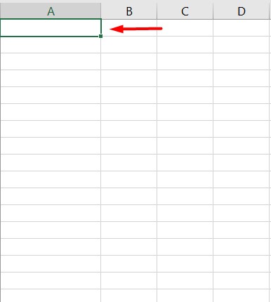
After you’ve identified your preferred column, click on the first empty cell of the column where you want to put the VLOOKUP function. Then, click the “Formulas” tab at the top of the screen. After that, click on the “Lookup and Reference” button on the ribbon. With this, a dropdown list will be shown from where you have to search for the VLOOKUP function. 

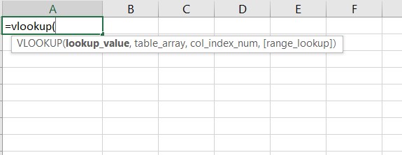
Select the “VLOOKUP” function from the dropdown list to start building your formula. After selecting the function, your highlighted cell in the spreadsheet will have the text “=VLOOKUP()” 

Another way to do this is to manually enter the formula into the cell, i.e., by typing “=VLOOKUP()” in it.

Now, do you remember the four different components of the formula discussed earlier? We need to fill those in the formula now.

Step-3: Specify the cell number where your lookup value is located

The very first component of the VLOOKUP formula is the piece of information in the spreadsheet that has data associated with it that you want the VLOOKUP function to search for and return to you. In other words, your lookup value.

So, in the formula, you have to specify the cell number of the lookup value for which you’re trying to find a match. Hence, if your lookup value is in the cell D2, your formula should look like: “=VLOOKUP(D2, [],[],[])”

---

Also Read: Become an Excel Pro in just 10 Formulas

---

Step-4: Specify the Table Array where your required data is located

The second component of the formula is the Table array or the range in which the required data is located. Enter the range of cells and the name of the sheet where your data is located in the table array field. 

Remember that, the sheet where your required data is located must be present in the Excel file that you’re working on. It’s not a problem if your data is in another sheet than what you’re working on, but it has to be in the same workbook.

For example, if your required data is located in “Sheet3” between cells D7 and K18, your table array entry should look like “Sheet3!D7:K18”.

 

Step-5: Enter the Column Index Number of the required data 

In this component, you have to specify the Column Number of the column where your required data is located. Here, the VLOOKUP function requires you to enter the order of the column in the range or table array, rather than its letter value.

For example, if your range or table array is column A through J (A: J), and your required values are in column J, then your column index number will be 10. This is because column J is the 10th column from the left in the range.

Step-6: Specify your Range Lookup to find either an Exact match or an Approximate match

In this component, you can specify whether you want the VLOOKUP function to look for an exact match or an approximate match. For searching an exact match, you need to enter False, and to find an approximate match, i.e., a value that is close to your lookup value rather than something identical to your lookup value, you need to ` enter True.

Step-7: Click Enter and fill the new column

Finally, to retrieve your desired data into the selected column from step 1, click enter. And voila! You can now view your desired data in the selected cell. Now, you can use your autofill handle to fill the rest of the column with your desired lookup values.

 

So, this is how you can use the VLOOKUP function to look up your desired values in your huge dataset, within seconds.

---

আমাদের কোর্সগুলোতে ভর্তি হতে ক্লিক করুন: 

• Microsoft Excel Course 
• Microsoft Office 3 in 1 Bundle
• Microsoft Word Course by Sadman Sadik
• Microsoft PowerPoint Course by Sadman Sadik

---

১০ মিনিট স্কুলের ক্লাসগুলো অনুসরণ করতে ভিজিট করুন: www.10minuteschool.com